What?
This is an article to remind me how to search a column in an Excel file for values found in another column (in this example, on another worksheet in the same workbook).

How?
So for demonstration purposes, I'm using a new Excel file with two worksheets called "Sheet1" and "Sheet2" respectively.

What I have:
A CSV file exported from Excel along with double-quotes

label1,label2
item1a,item2a
item1c,"item2c,c"
item1b,item2b

What I want:
To read the file (stored on the server) and convert to a JavaScript array of objects

var my_object_array = [
     { my_col1_val: 'item1a', my_col2_val: 'item2a' },
     { my_col1_val: 'item1b', my_col2_val: 'item2b' },
     { my_col1_val: 'item1c', my_col2_val: 'item2c,c' }
];

What I want again:

• Read a CSV file already uploaded with JavaScript
• Populate a JS array with each row
• Account for strings containing double-quotes (and commas to ignore)
• Sort the resulting object array

How?

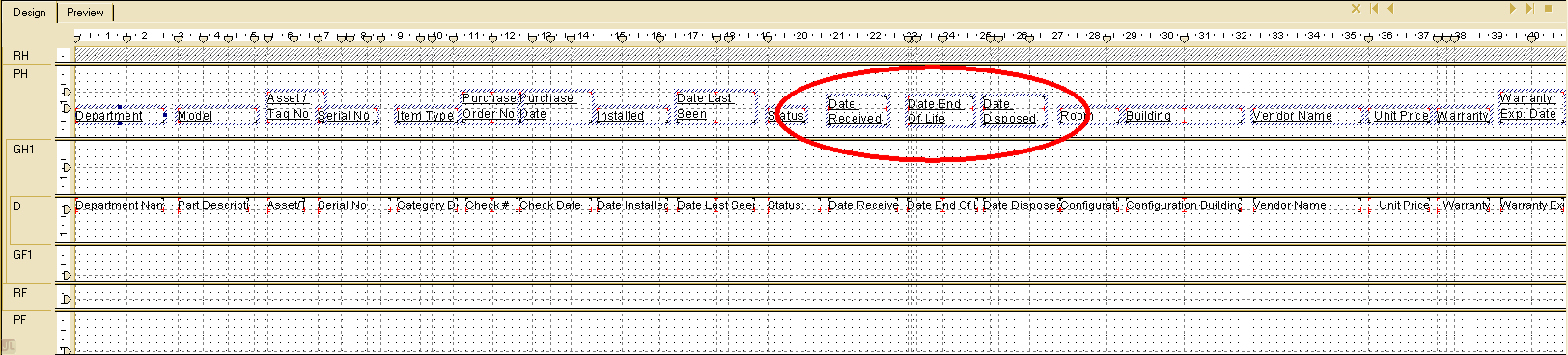
If you've been to the point where you're exporting a report to Excel, and only some of the column headers appear, then try this:

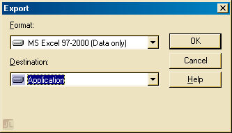
I googled this for ages and found different suggestions here and there but none of them produced consistent results.  One solution was to untick "Simplify page headers" on the Excel Format Options when you export the report.  Because our report is exported via a web-based system, this extra dialog doesn't appear when our users export their reports.  Not that it solved it as only some different headers appeared on the exported report when we followed that suggestion.

Consider the following report in design view, only the circled headings would appear on the exported report:

So I googled this for a while and there are a lot of solutions out there, none of which applied to what we meant and lots of people in the same boat.

The Situation
We have an Excel report which summarizes for our guys at the top, all the activities and time spent by staff. There are several filters available on the report (only a few to keep it simple silly). When you click on the filter, a dropdown appears with all available values listed.

The Problem
The values are listed in alphabetical order at first. If any new values come along then they get added to the bottom of the list... This is the problem. For example, if the year dropdown has a list of 2010, 2011, 2013; then if you add an entry which has year 2012, then the dropdown list will be in the following order: 2010, 2011, 2013, 2012.

The Solution

The Situation
I have a Microsoft Excel 2007 file that connects to a SQL Server 2008 R2 database. The Excel file pulls data using lookup tables and displays the data in an Excel Spreadsheet.

The Problem
We can select all cells and set row height to be 30 for example, but everytime we refresh the data in the Excel spreadsheet, all the rows get re-adjusted to fit the data and lose that consistency.

A Workaround: New line inserted before and after
So this is where I am at the moment without VBCode and other suggestions. Instead I add a newline in front of and after the smallest data value (one that I know will never be two lines (or two words)) within the SQL query itself. We have a DEPT column that is an acronym of the departments so for example:

Thought I'd put a quick note here, I tried a fair few solutions that didn't work and then found this hidden away in a forum:

Quick Count

=INT(SUMPRODUCT((A3:A1000<>"")/COUNTIF(A3:A1000,A3:A1000&"")))

This returns the number of unique values in the range A3 to A1000 and excludes the blank/empty cells.

Display all Unique
Found this note on one of Microsoft Help sites:

What?
We have an excel spreadsheet which reports against a mySQL database and reads time spent on projects by IT Service colleagues. The main report is a pivot table with staff members along the top, tasks down the first column, and time spent in the form of person days in the cross-join.

Why?
Currently the smallest bookable time by low-level tape monkeys and techies is 30 minutes (Managers it would appear can book whatever time, eg. 5mins). 30 minutes for us translates to 0.07 in person days (a person day being 7 hours and 24 minutes or 26640 seconds).

How?

What?
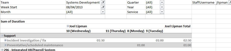
This is a quick note to myself so that I never use parentheses in the column headings again. Basically I have a pivot table in Microsoft Excel 2010 with the projects down the left (in the first column) and the days of the week along the top.

Why?
The excel report would hit a bug where it couldn't work out that 10 (Wednesday) happened after 8 (Monday).

How?
See the following screenshot and note the dates for Monday, Tuesday, Wednesday, and Thursday: